Linear programming is an algorithm that solves the general problem of maximizing a linear outcome given linear constraints. This includes the very broad category of problem "given a limited amount of resources and objectives using those resources, how can I output objectives to maximize value?". What exactly does this mean and how can we solve these kinds of problems? Let's go over it, using skating downhill as an analogy to help us understand both what these problems look like and how to find optimal solutions for them.

ToC

• Example linear programming problem with terms
  • Constraints
  • Optimality function
  • Solutions and feasible solutions
  • Feasible region
• The feasible region as a skating rink
  • Two key properties of linear programming problems
• Skating our way to the solution
  • Picking a starting point
  • Skating downhill
  • The entire skating process
• Creating variables to represent leftover ingredients
  • Using basises to pick corners
• Formalizing our skating through math
  • Step 1: picking an initial basis to start at
  • Step 2.1: Finding a constraint to push off of
  • Step 2.2: Figuring out where we will land
  • Step 2.3: Landing gracefully at our new basis
  • Step 3: returning the solution
• Conclusion

Example linear programming problem with terms

As an example problem, we will try to figure out how much ale and bread we should produce given a limited amount of ingredients to maximize profits.

Take the following tables listing the recipes of ale and bread, their selling prices, and the amount of ingredients we have.

Constraints

The constraints in this problem, given the amount of ingredients we have and how much ingredients you need to produce ale and bread , are the following:

Each constraint makes sure we don't use more of any ingredient than we have. Additionally, we also constrain on producing a nonnegative amount of either product.

Optimality function

The optimality function for a problem describes the value of a solution, in this case, the amount of profit we make . Given sells for 4 and for 5:

Solutions and feasible solutions

A solution would consist of the amount of and you want to produce. A feasible solution is one that satisfies our constraints.

For example, some feasible solutions for this problem:

• : uses 2 corn, 5 wheat, 3 sugar
• : uses no ingredients

and some infeasible solutions:

• : we can't produce negative of a product
• : uses 16 wheat, more than the 12 we have

Feasible region

The set of feasible solutions for a problem is called the feasible region.

The feasible region as a skating rink

To illustrate how linear programming works, we will use a skating rink as an analogy. In this scenario, an inclined plane will represent our solution space, with the incline of the plane matching the optimality function. Lower down represents more optimal/profitable solutions.

Ideally we would skate down hill forever and make infinite money. However, each of our constraints divides our plane into a feasible section of solutions and an infeasible section. Because each of our constraints are linear and divide our solution space using straight lines, they combine to section our hill into a convex polygon of feasible solutions: the feasible region, aka our skating rink:

We'll use the term "constraint" to equivalently mean the borders depicted above through this article.

When will the feasibility region be a convex polygon?

Linear constraints will generally lead to one of 3 cases:

1. An unbounded feasible region, like our region above before we add the 3rd constraint. No guaranteed optimal solution as we may be able to continue in a direction forever.
2. A feasible region that is a convex polygon. Always solvable using linear programming.
3. No feasible region. This could occur if we added in a constraint that covered our entire feasible region. No solution in this case.

What does "linear" mean exactly?

"Linear" in math describes an equation where variables have only constant coefficients:

• Linear:
• Linear:
• Not linear:
• Not linear:

Our example problem is linear as the amount of ingredients used and the profit we make scales linearly with the amount of products produced, allowing us to express each part of the problem as a linear expression. If something funky happened like the profit per product going down with higher production (maybe you satisfy all the demand for bread), linear programming would not be applicable. Knowing a problem is linear makes it easier to solve.

Two key properties of linear programming problems

Because our feasible region is a convex polygon, and because the optimality function leads in a constant direction (down hill) no matter where are, we can realize two important properties of our feasible region:

1. The optimal solution will always be at one of the corners. If we are in the middle of the feasible region or on a constraint, we can just continue to slide down slope to a corner of the region get to a more optimal solution.
2. We will never get stuck in an inset portion of the region moving downhill unless it is the optimal solution. This is due to the region being convex.

If we were to drop a ball anywhere in our rink, it would naturally fall down to the optimal point due to the above properties:

The linear programming algorithm will involve traveling downhill along the perimeter of the feasible region until we can travel downhill no further, at which point we know we are the optimal solution.

Skating our way to the solution

Picking a starting point

To find an optimal solution, we will use as a starting off point any corner of the feasible region, grabbing onto both the constraints forming the corner. We will start at as it is an easy corner to come up with.

Skating downhill

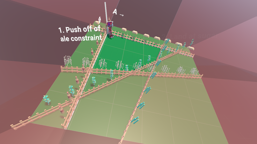
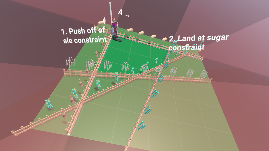
From our starting point, we will travel downhill along constraints until we land at the lowest corner. Each step of our process will involve the following:

1. Pick a constraint we are holding onto that we can push off of to go downhill. If we can push multiple ways to go downhill, we can choose either direction arbitrarily, as moving downhill in any direction is bringing us closer to the solution and we don't need to worry about getting stuck in a non-optimal corner.
2. Figure out which corner we will land at after pushing.
3. Push off the constraint and land gracefully at the new corner.

We continue to do the above until we can no longer travel downhill by pushing off of a constraint, which will only happen after arriving at the optimal solution.

The entire skating process

Our process then is the following:

1. Pick an initial corner of the feasible region to start at.
2. Continue to do the following as long as you can travel downhill:
   1. Pick a constraint that we can push downhill off of.
   2. Figure out where we will land after pushing off.
   3. Push off the constraint and land at the new corner.
3. Return the final corner we have landed at as the solution.

Creating variables to represent leftover ingredients

Before we can begin to formalize our skating algorithm, we need to do one step to redefine how we look at our problem. Currently, our constraints are described as inequalities in terms solely of and :

• Corn:
• Wheat:
• Sugar:
• Ale:
• Bread:

However, this formulation does not make it easy to pick corners of the feasible region, which we would like to do as we know our solution is at one of the corners. To facilitate picking corners, we will introduce new variables representing how much of each ingredient we have leftover to do this.

We will use as variables representing our leftover corn, wheat, and sugar, and redefine our inequalities as equalities involving leftovers. For example, means "The amount of corn we're using to produce ale and bread, plus the amount of leftover corn, is equal to our total corn available."

The entire formulation of our problem now looks like the following:

Constraints

• Corn:
• Wheat:
• Sugar:

Optimality Function

In future formulations, we will omit that our variables must be nonnegative and just keep in mind that this is the case.

Using basises to pick corners

Having variables representing the leftover of each ingredient now means they represent our distance from the constraints: when the leftover amount of an ingredient is 0 we are on the constraint representing it. This makes it easy to select a corner of our feasible region (where two constraints intersect) by setting any two of our variables two zero.

We call a choice of two variables we set to 0 arrive at a corner a basis, with each basis corresponding to a corner of the feasible region. More generally, a basis could also represent the intersection of two constraints outside of the feasible region, but we will be careful to stay on the perimeter of the feasible region while skating. Visible basises are labeled below, with feasible ones being labeled green and unfeasible ones red:

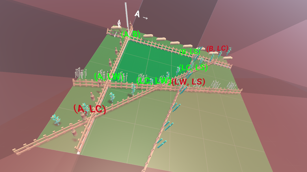
Similar to using "constraint" to refer to an edge, we will also here use "basis" to refer to a corner of the feasible region through the rest of this article.

Formalizing our skating through math

Given our skating process, let's formalize it using an actual algorithm.

Step 1: picking an initial basis to start at

For our problem instance:

We need to zero out 2 variables to choose an initial basis to start at. Using basis gives us a very obvious and obviously feasible solution of the remaining variables, so we will start with those (although you could zero out others if you want to start somewhere else).

We will indicate which variables are currently in our basis by surrounding them with brackets:

• Basic variables:

Resulting in the following values for all our variables:

• Basis variables (must be 0):
• Non-basis variables:

Great, we have a solution! However, the issue with this solution is it is not optimal as we are not making any money.

Step 2.1: Finding a constraint to push off of

Looking at our optimality function

We would rather not zero out the ale and bread we produce as they contribute to our profit: right now we aren't making any money with both being 0. It would be better to zero out something like leftover corn, which according to the optimality function doesn't make us any money.

To move towards a more optimal solution, we look at the optimality function to find a variable with a positive coefficient, indicating it would be more profitable to not be 0. We then "push off" of the constraint for it by making it non-0, sliding along the other constraint we keep in the basis.

We can choose to take either or out of the basis now, but let's arbitrarily choose . Now, we need to figure out which constraint we will land at after pushing off of the constraint.

Step 2.2: Figuring out where we will land

The further we move from the constraint after pushing off, the larger the value of is. Thus, we can find the first constraint we run into when sliding along the constraint by finding the other constraint whose intersection with is at the smallest value of .

Finding the intersection of the constraint with another constraint can be done by setting both their variables to 0. Looking at our system

We get the following values for when we set and another variable to 0.

1. Basis of :
2. Basis of :
3. Basis of :

We see here that the basis gives the smallest value for A, so we know is the first basis we encounter as we slide along the constraint.

Step 2.3: Landing gracefully at our new basis

We have figured out the new basis we will land at: .

Now all we need to do is reformulate our system of equations to make steps 2.1 and 2.2 easy to repeat.

Step 2.1 was easy because the optimality function made it obvious how our basis variables contributed to our profit, and we would like this to again be obvious for our new basis. To achieve this, we will use elimination to remove our now non-basis variable from our current phrasing of the optimality function, replacing it with our new basis variable to get an optimality function in terms only of our basis variables:

−
¯¯¯¯¯¯¯¯¯¯¯¯¯¯¯¯¯¯¯¯¯¯¯¯¯¯¯¯¯¯¯¯¯¯¯¯¯¯
¯¯¯¯¯¯¯¯¯¯¯¯¯¯¯¯¯¯¯¯¯¯¯¯¯¯¯¯¯¯¯¯¯¯¯¯¯¯

Now two things are obvious again:

1. Our profit given both and being 0 is 12. Better than our profit of 0 from before, our process is working!
2. would not contribute to the profit as it is negative in the optimality function. However, still would contribute to our profit as it is positive: this is the constraint we will want to push off of next.

We can use the same process to simplify our other equations:

Simplifying the other equations

Given our equations

−
¯¯¯¯¯¯¯¯¯¯¯¯¯¯¯¯¯¯¯¯¯¯¯¯¯¯¯¯¯¯¯¯¯¯¯¯¯¯

−
¯¯¯¯¯¯¯¯¯¯¯¯¯¯¯¯¯¯¯¯¯¯¯¯¯¯¯¯¯¯¯¯¯¯¯¯¯¯

¯¯¯¯¯¯¯¯¯¯¯¯¯¯¯¯¯¯¯¯¯¯¯¯¯¯¯¯¯¯¯¯¯¯¯¯¯¯

Step 3: returning the solution

Repeating step 2 twice more to get to the optimal solution

We repeat step 2 two more times to get to the optimal solution. First, because B is positive in the optimality function, taking B out of the basis and LC in to get to:

and then, because LS is now positive in the optimality function, taking LS out of the basis and LW in to get:

Eventually, we reach a form of the optimality function where none of the variables in the basis are contributing to the profit, at basis .

This means we are most optimally producing products by using up all of our corn and wheat, with some sugar remaining that we don't do anything with. We can return the current values we have as our optimal solution:

Conclusion

Hopefully our skating analogy made it clear what linear programming is doing: navigating downhill (in the direction of the optimality function) along edges of the feasible region (constraints), evaluating corners (basises) of the region until we reach a point where we can't go downhill any further (the optimal solution). While the implementation of the algorithm itself can seem be a bit cumbersome (mainly our step to reorganize stuff), in reality what it's doing is quite simple: moving downhill along the edges until it gets to the solution.

Applying linear programming in higher dimensions

Because our example problem had only two objectives (ale and bread), this resulted in two axes of our solution space, making the problem two dimensional. Very often though, we will have more that two objectives. Even in higher dimensions, the process would still be the same: follow the objective function along constraints towards corners of the feasible region until we can't follow it any further. In this case, the feasible region would not be a 2d polygon but a multidimensional polytope, but there's no reason why our algorithm would break in higher dimensions.